In the context of stationary sensor networks, our goal is to use spatio-temporal correlations inherent to traffic data to reduce the maintenance costs of the monitoring infrastructure. We aim to minimize communication incurred by the propagation of traffic data from a temporary deployment of stationary sensors to the Traffic Monitoring Centre (TMC) gateways. Such a temporary deployment is meant to support applications utilized for future planning decisions by local authorities.This class of applications does not require the most recent traffic information about the network, so we are focusing on periodic traffic data propagation with a report period that is much larger than the sensing period.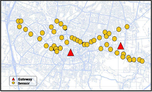
We assume a network architecture that includes two types of nodes: sensor nodes and gateway nodes. Sensor nodes can be equipped with a variety of sensors. In this work we assume sensor nodes are set up to measure traffic flow (cars/time). We assume that sensor nodes communicate over wireless links with neighbouring nodes in their range in order to relay data towards a gateway node. In the temporary deployment we are considering, we expect most, if not all, sensor nodes to be battery powered devices that have limited storage and processing capabilities. Gateway nodes collect readings from sensor nodes. We consider them to have a fixed power source, unlimited bandwidth, storage and processing capabilities, and relay data to the TMC where the traffic monitoring applications are running. We have based our analysis on a real traffic dataset generated by an inductive loop deployment in the city of Cambridge. It consists of traffic flow readings provided every 5 minutes. We therefore assume that each sensor node produces a time series of flow readings with the same frequency.
Each node locally produces a large time series of traffic data per period, which, if propagated in an uncompressed form, would require a large number of transmissions. Assuming tolerance for a small error in the reported data, we examine lossy signal compression based on a prominent signal processing technique, the Fast Fourier Transform (FFT), and we evaluate its efficiency in reducing communication.
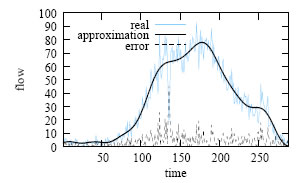 After the application of FFT, we compress by retaining only a certain number of Fourier coefficients so that our time series can be approximated with the desired error. Figure~\ref{figure:fouriermse} shows the time series approximation obtained when only the first 15 coefficients are used, which require $n*sizeof(float)$ bytes of memory. The first FFT coefficients correspond to the lower frequencies of the signal which account for the major signal variations. The figure on the left shows the Fourier approximation of 24 hours of time series data (288 integer flow values). The approximation signal is constructed from 15 coefficients of type float which, in the sensor platform, are equivalent to 30 integers. The compression ratio achieved here is 89.6%. FFT is an attractive choice since it mostly utilizes integer operations, making it easier to compute in resource-constrained nodes where dedicated floating point hardware is typically absent.
To explore opportunities for further compression, we exploit the correlation between two time series of the same node on different dates (temporal corelations) and the correlation between two time series of different nodes on the same date (spatial correlations). In the real traffic dataset, we observed that For for more than 80% of the sensors, their daily readings are highly correlated with those in one of the previous seven days. The FC-Temporal algorithm exploits those:
Each sensor node running FC-Temporal tries to compress today's time series locally, by expressing it as a linear function of a previous day's time series. The red sensor node on the left, checks whether today’s time series is correlated with a time series in the previous week. It chooses Friday as the one that is highly correlated, and expresses today’s time-series as a linear combination of the time-series of Friday that the gateway already knows. Subsequently the regression parameters a and b as well as an identifier for the day Friday are forwarded to the gateway. The gateway is able to reproduce today's approximation using the regression parameters and the time-series data that was stored on Friday.
We exploit spatial correlations in a similar manner, reducing time-series data to regression parameters at intermediate nodes on the path to the gateway.